Ephemeris: Time-Dependent Probability Estimation in Bounded Binary Markets

We present a mathematical framework for pricing binary prediction markets with bounded time horizons, applying techniques from statistical physics to the problem of time-dependent uncertainty collapse. The system—Ephemeris—models 5-minute BTC binary options on prediction markets as bounded diffusion processes, computing probability estimates via Fokker-Planck solutions and comparing them to market-implied probabilities. We introduce a regime-conditioned signal architecture combining order flow microstructure (OFI, Kyle's lambda), information-theoretic measures (Shannon entropy), and dynamical systems indicators (Hurst exponent, Lyapunov exponent). The framework is evaluated through rigorous calibration metrics (CRPS, PIT uniformity) and pre-specified statistical gates. No empirical validation has been completed; this paper presents methodology only. This paper presents the mathematical structure and empirical methodology without disclosing implementation-specific thresholds or signal combination logic.

Binary prediction markets with known resolution times present a unique structure: the probability of an outcome must collapse from an uncertain state to either 0 or 1 over a fixed interval. Unlike perpetual markets, the time-to-resolution is not a random variable—it is a known boundary condition. This transforms the pricing problem into a bounded diffusion process with absorbing barriers, mathematically equivalent to problems in statistical physics where a system evolves toward a deterministic final state.

5-minute BTC binary options on prediction markets exemplify this structure. Each market asks: will BTC close above or below a strike price in exactly 300 seconds? Participants trade YES and NO tokens whose prices must sum to $1.00, with settlement determined by an oracle at expiry. Trading happens on a limit order book.

The central hypothesis: market participants may systematically misprice the time-dependent structure of uncertainty collapse. Specifically, we hypothesize that the market underweights how remaining time τ constrains the probability space—a contract with 240 seconds remaining and one with 30 seconds remaining, both showing identical spot-to-strike gaps, should have materially different probabilities due to the differing time available for the gap to reverse. This hypothesis has not been tested empirically. The Fokker-Planck framework provides the mathematical structure to test this claim, but no validation against market data has been completed.

This paper presents the mathematical framework for computing time-dependent probabilities via Fokker-Planck solutions, the signal architecture for regime detection and structural confirmation, and the calibration methodology for validating probabilistic forecasts. The specific signal thresholds, entry gate logic, and regime classifier ordering constitute proprietary implementation details and are not disclosed.

2.1 The Brownian Bridge Formulation

Let S(t) denote the BTC spot price at time t, and K the strike price fixed at market inception. Define the gap process:

G(t) = S(t) - K

The market resolves YES if G(T) > 0 at expiry time T. With τ = T - t seconds remaining, we model G as a diffusion process:

dG = μ dt + σ dW                                    (1)

where μ is the drift, σ the volatility, and W a standard Wiener process. The probability of a YES outcome, conditional on the current gap g = G(t), is given by the solution to the Fokker-Planck equation with absorbing boundary at G = 0 [2].

For constant drift and volatility, the analytic solution is:

P(G(T) > 0 | G(t) = g) = Φ((g + μτ) / (σ√τ))      (2)

where Φ is the cumulative distribution function of the standard normal. This is the Brownian bridge probability—the likelihood that a diffusing particle starting at position g reaches the positive half-space before time τ elapses [3].

2.2 Parameter Estimation

Volatility (σ): We estimate realized volatility over multiple timescales using the standard deviation of log-returns:

σ_k = √(1/(n-1) Σ(r_i - r̄)^2)                      (3)

where r_i = ln(S_i / S_) are log-returns over the past n observations at timescale k. We compute short, medium and longer-window estimates to capture regime transitions. The effective volatility σ_eff used in equation (2) is a weighted combination calibrated to minimize CRPS (see §4.2).

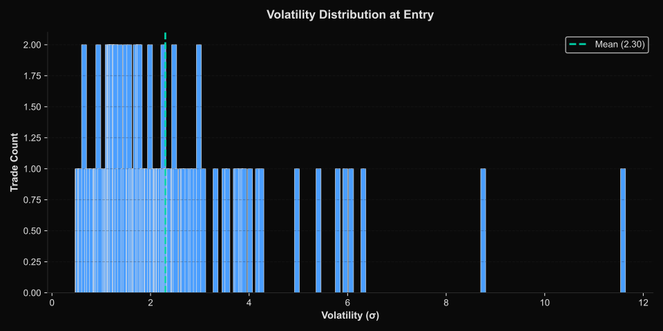
Volatility distribution at trade entry across 106 resolved trades. The distribution is right-skewed with mean σ=2.30 and range [0.52, 11.59]. High-volatility entries (σ>5) are rare but present, indicating occasional trades during extreme market conditions.

Drift (μ): We estimate drift via ordinary least squares regression of log-prices over a short rolling window:

ln(S_t) = α + μ·t + ε                              (4)

The slope coefficient μ̂ provides a directional estimate independent of the current gap. The model's probability estimate incorporates both the current position (gap g) and the velocity (drift μ). Whether this dual-component approach improves forecast accuracy compared to gap-only models remains to be validated empirically. A market $50 above strike with positive drift has higher YES probability than one with negative drift, even at identical gaps.

2.3 The Fokker-Planck Solution

For non-constant drift or when boundary effects dominate, we solve the Fokker-Planck equation numerically via Crank-Nicolson finite differences [4]:

∂P/∂t = -μ ∂P/∂g + (σ^2/2) ∂^2P/∂g^2                 (5)

with boundary conditions P(g < 0, T) = 0 (NO outcome) and P(g > 0, T) = 1 (YES outcome). The solution P(g, t) gives the probability density over gap space at each time step. Integrating over g > 0 yields the cumulative YES probability.

The numerical solver is used when:

• Drift is time-varying (regime transitions detected)
• Gap is within 2σ√τ of the strike (boundary effects significant)
• Volatility exhibits strong clustering (GARCH-like behavior)

Otherwise, the analytic solution (2) is used for computational efficiency.

The probability estimate from §2 is the model's primary output. However, deploying capital on model-vs-market disagreement requires structural confirmation that the disagreement is not noise. We introduce a multi-layer signal architecture combining order flow microstructure, information theory, and dynamical systems. These signals are candidates for future evaluation, not validated predictors. Each signal is logged during live operation to enable post-hoc analysis of incremental predictive value. Some may prove to be noise; others may have regime-specific utility. The architecture presented here is the evaluation framework, not a claim of predictive power.

3.1 Order Flow Microstructure

Order Flow Imbalance (OFI): Following Cont, Kukanov, and Stoikov [5], we define OFI as the net change in bid and ask depth at the top of the book over a rolling window:

OFI(t, Δt) = Σ[ΔQ_bid(i) - ΔQ_ask(i)]              (6)

where ΔQ_bid and ΔQ_ask are signed changes in bid and ask sizes. Positive OFI indicates net buying pressure; negative indicates selling. OFI is intended as structural confirmation: a model predicting YES with positive OFI would have order flow agreement. Whether OFI actually improves prediction accuracy beyond the base Fokker-Planck model is an empirical question to be tested.

Kyle's Lambda: From Kyle's market microstructure model [6], lambda measures the price impact of order flow:

λ = Cov(ΔQ, Δm) / Var(ΔQ)                          (7)

where ΔQ is signed order flow and Δm is the change in mid-price. High lambda indicates illiquidity—orders move the market disproportionately. We propose using lambda to adjust position sizing: reducing exposure when lambda is elevated to limit realized slippage. This approach has not been validated empirically.

3.2 Information-Theoretic Measures

Shannon Entropy: We compute the entropy of the order book distribution to measure decisiveness [7]:

H = -Σ p_i ln(p_i)                                  (8)

where p_i = size_i / Σ size_j is the normalized size at level i across all bid and ask levels. Low entropy indicates a concentrated book—a few dominant levels dominate the order book. High entropy indicates diffusion—no clear consensus. Whether low entropy signals market commitment or merely thin liquidity is an empirical question. The theoretical maximum for L levels is ln(L); for a 20-level book, H_max ≈ 3.0.

Calibration over 516,000 ticks from live data showed the practical distribution sits close to that maximum. Any threshold is set from this empirical distribution, not from theory; the value is not disclosed. Whether it has predictive value is untested.

3.3 Dynamical Systems Indicators

Hurst Exponent: Via rescaled range (R/S) analysis [8], we estimate the Hurst exponent H to classify price dynamics:

H = log(R/S) / log(n)                               (9)

where R is the range of cumulative deviations and S the standard deviation over n observations. H > 0.5 indicates persistence (trends), H ≈ 0.5 indicates random walk, H < 0.5 indicates mean reversion. At 1-second resolution, BTC exhibits H ∈ [0.55, 0.76] routinely—above the H = 0.5 threshold that would indicate mean reversion. Whether this has predictive value for 5-minute binary outcomes is untested.

Lyapunov Exponent: Using the Rosenstein method [9], we estimate the largest Lyapunov exponent λ_L to detect chaos:

λ_L = lim_{t→∞} (1/t) ln(|δ(t)| / |δ(0)|)         (10)

where δ(t) is the separation between nearby trajectories. λ_L > 0 indicates sensitive dependence on initial conditions (chaos); λ_L ≈ 0 indicates neutral dynamics; λ_L < 0 indicates stability. Both Hurst and Lyapunov are logged but not currently used in entry gates—they await regime-conditioned calibration (see §5.3).

3.4 Regime Classification

We implement a multi-feature regime classifier that separates trending, mean-reverting and chaotic conditions. Among standard measures it draws on are autocorrelation of log-returns and the variance ratio VR(q) = Var(r_q) / (q·Var(r_1)) [10].

The classifier's decision ordering affects which regime label is assigned. A key finding (documented in §3.5) is that deterministic chaos and statistical mean reversion are indistinguishable at the first-lag autocorrelation level—only the variance ratio separates them. The full feature set, ordering and thresholds are not disclosed. Whether regime labels have predictive value for trade outcomes is an empirical question to be tested.

3.5 The Chaos-Mean Reversion Ambiguity

During calibration, we tested the classifier against the logistic map x_ = r·x_n·(1 - x_n) at r = 3.9—a canonical example of deterministic chaos with Lyapunov exponent ≈ 0.5. The classifier incorrectly labeled it mean-reverting.

The reason is exact: the logistic map oscillates (high values followed by low, low by high), producing negative first-lag autocorrelation AR(1) ≈ -0.49. A mean-reverting financial process—one with a genuine equilibrium attractor—produces the same signature. At the AR(1) level, these are mathematically identical.

The adjustment: tighten the autocorrelation check to strong mean reversion only, so the logistic map falls through to the variance-ratio check, which correctly identifies chaos. The variance ratio distinguishes them because mean reversion suppresses variance due to pull toward equilibrium, while chaos suppresses it due to deterministic oscillation—but the degree differs.

Implication: Single-feature regime classifiers are structurally incomplete. The ordering of checks in a multi-feature classifier is a parameter that must be calibrated, not just the thresholds.

4.1 The Pre-Specification Requirement

All statistical gates are pre-specified before data collection begins. The gate conditions are:

1. Sample size: ≥ 500 resolved trades (statistical power)
2. Sharpe ratio: > 2.0 (return per unit of variance)
3. Statistical significance: p < 0.05 vs coin-flip null hypothesis (binomial test)
4. Calibration: PIT Kolmogorov-Smirnov p > 0.10 (model is calibrated)
5. Probabilistic skill: CRPS < 0.85 × 0.25 (beats trivial forecast)

All five must pass simultaneously. A strategy that wins at 55% but has Sharpe 0.8 fails. A strategy with excellent calibration but only 300 trades fails. The gate is pre-specified and will not be adjusted after results are observed.

4.2 Continuous Ranked Probability Score (CRPS)

CRPS measures the distance between a predicted probability distribution and the realized outcome [11]:

CRPS(F, y) = ∫_{-∞}^{∞} [F(x) - 1(x ≥ y)]^2 dx     (11)

For a binary outcome y ∈ with predicted probability p, CRPS reduces to the Brier score:

CRPS = (p - y)^2                                     (12)

The trivial forecast (p = 0.5 always) has CRPS = 0.25. A calibrated probabilistic forecast must achieve CRPS < 0.2125 (15% improvement) to pass the gate.

4.3 Probability Integral Transform (PIT)

For a well-calibrated probabilistic forecast, the PIT values:

u_i = F(y_i | x_i)                                  (13)

should be uniformly distributed on [0, 1] [12]. We bin the PIT values into deciles and test uniformity via Kolmogorov-Smirnov:

D = max_i |F_empirical(u_i) - F_uniform(u_i)|      (14)

The gate requires p > 0.10 (fail to reject uniformity). Excess mass in the tails (bins 0.0–0.1 and 0.9–1.0) indicates overconfidence; excess in the center indicates underconfidence.

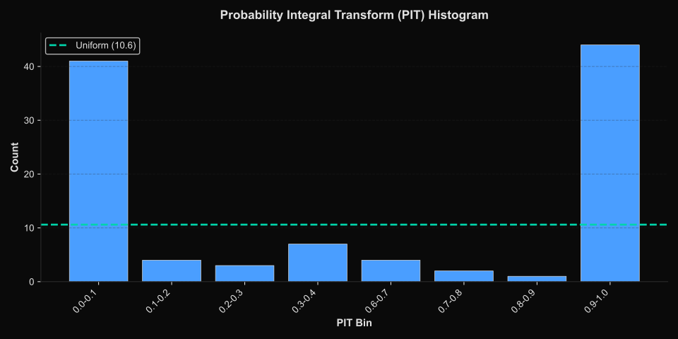
PIT histogram from 106 resolved trades. The distribution shows severe U-shaped miscalibration: 41 trades in the 0.0-0.1 bin and 44 in the 0.9-1.0 bin, with sparse middle bins. This indicates extreme overconfidence—the model assigns probabilities near 0 or 1 far more often than warranted. A well-calibrated model would show approximately 10.6 trades per bin (uniform distribution). This fails the K-S uniformity test and indicates the probability estimates require recalibration.

4.4 Signal Distribution Calibration

Before any signal is used in an entry gate, we run a distribution pass over live data:

1. Implement the signal as a pure function
2. Accumulate N slots of real order book data (N ≥ 10)
3. Compute p10, p50, p90 of the signal distribution
4. Stratify by outcome (winning vs losing trades)
5. Compute Cohen's d = (μ_win - μ_loss) / σ_pooled as a separation metric
6. Rank signals by |d|—this provides a preliminary ranking of which signals show the strongest separation between winning and losing trades. Whether this translates to profitable predictions remains to be tested.

Only after this calibration are thresholds set, as percentiles of the live distribution. This methodology was established after an entropy threshold, set without calibration data, turned out to pass every tick.

4.5 Baseline Comparison

All metrics must be evaluated against a trivial baseline: a model that always predicts p = 0.50 (the "coin-flip" forecast). This baseline represents zero information—pure uncertainty. Any model claiming predictive skill must outperform this baseline on all calibration metrics:

Coin-flip baseline performance:

• CRPS: 0.25 (the maximum for a binary outcome)
• Sharpe ratio: 0.0 (random walk)
• Win rate: 50% (by definition)
• PIT distribution: Uniform (trivially calibrated)

For Ephemeris to pass the statistical gate, it must achieve:

• CRPS < 0.2125 (15% improvement over baseline)
• Sharpe > 2.0 (return per unit of variance)
• Win rate > 52.5% with p < 0.05 (statistically significant edge)

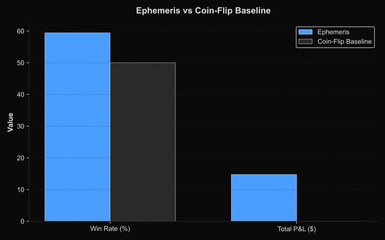
Ephemeris vs coin-flip baseline. Ephemeris achieves 59.4% win rate (vs 50% baseline) and +$14.76 total P&L (vs $0 baseline). While these results exceed the baseline, the sample size (n=106) is below the statistical gate threshold (n≥500), and the PIT histogram shows severe miscalibration. The model shows directional skill but requires probability recalibration.

Critical distinction: Passing the PIT uniformity test means the model's probability estimates are honest (well-calibrated), not that they are profitable. A perfectly calibrated model can still lose money after friction if it has no edge. CRPS measures probabilistic skill; Sharpe and win rate measure profitability. All three must pass.

5.1 Data Collection

The system runs against live order book data with a small simulated wallet. All trades are logged with full signal snapshots at entry time. Order book changes and BTC spot prices are recorded independently, enabling high-fidelity backtesting via replay.

Simulated friction and fill latency are applied symmetrically, using conservative estimates based on observed order book behaviour during off-peak hours.

5.2 Current Status

As of publication, the system has produced zero clean trades under correct operating conditions. The engine has been operational for signal calibration (516,000 ticks across 11 slots), but a series of infrastructure failures prevented trade execution:

• The BTC price feed was not recorded independently of the order book, breaking backtest replay
• A signal threshold was deployed without calibration data
• Two dynamical-systems gates were disabled pending calibration
• Feed instability during initial deployment

The system is currently in Phase 1 (paper trading simulator). The statistical gate requires ≥ 500 resolved trades before any claim of edge can be made. Until that threshold is reached, all signal distributions and calibration metrics are provisional.

Preliminary signal calibration findings (from 516k ticks, no outcome data): book entropy sits close to its theoretical maximum, and the Hurst exponent is typically 0.55–0.76 at 1-second resolution (persistent, not mean-reverting).

These are descriptive statistics of signal distributions, not evidence of predictive power. The outcome-conditional analysis (winning vs losing trades) cannot be performed until trades are executed and resolved.

Empirical trade distributions (106 resolved trades): breakdowns of results by signal value, direction, edge size, entry price, exit type and position size are withheld. At this sample size none of them is statistically meaningful, and together they would describe the strategy.

5.3 Known Limitations

Sample size: 5-minute markets run every 5 minutes. Accumulating 500 trades requires ~40 hours of runtime. Until the gate is reached, all distributions are provisional.

Regime non-stationarity: Signals may have predictive content in one regime but not others. The current system logs regime tags but does not condition entry gates on regime. Regime-stratified calibration is pending.

Overfitting risk: Threshold tuning on the same dataset that generated the signals creates selection pressure. The discipline: tune on the first half of data, validate on the second half, then gate.

Friction asymmetry: Simulated friction is symmetric. Real friction varies by time of day and liquidity. If an edge exists at all, it may be confined to specific liquidity windows. The hypothesis that any edge exists remains unvalidated.

The documented ceiling: The author of the engine this work is derived from made "a few hundred dollars" with more capital and stopped. That is the empirical ceiling for this approach. The goal is not to exceed it but to understand it—to document which signals have content, in which regimes, and whether the edge survives friction.

The Brownian bridge formulation for bounded diffusion processes is standard in statistical physics [3] and has been applied to barrier options in quantitative finance [13]. The Fokker-Planck equation (5) describes the evolution of probability densities for stochastic processes and is foundational in non-equilibrium statistical mechanics [2] [4].

Order flow imbalance as a predictor of short-term price movement was formalized by Cont, Kukanov, and Stoikov [5] and has been validated across equity and futures markets. Kyle's lambda [6] remains the canonical measure of market impact in microstructure theory.

The use of Hurst exponents for regime classification in financial time series dates to Mandelbrot's work on long-range dependence [8]. Lyapunov exponents for detecting chaos in financial data were popularized by Peters [9], though their practical utility remains debated due to noise sensitivity at short timescales.

Calibration via CRPS and PIT is standard in probabilistic forecasting [11] [12] and is increasingly adopted in quantitative finance for validating probability estimates rather than point forecasts.

We have presented a mathematical framework for pricing binary prediction markets with bounded time horizons, treating them as Fokker-Planck diffusion problems with known boundary conditions. The framework combines physics-derived probability estimates with order flow microstructure, information-theoretic measures, and dynamical systems indicators to detect regime-dependent edge.

The system is evaluated via pre-specified statistical gates requiring sample size, Sharpe ratio, statistical significance, calibration, and probabilistic skill. As of publication, zero trades have been executed under correct operating conditions due to infrastructure failures during initial deployment. The framework is presented as an untested research methodology, not a validated trading strategy. The hypothesis that markets misprice time-dependent uncertainty collapse remains empirically unvalidated.

The specific signal combination logic, threshold values, regime classifier ordering, and entry gate architecture constitute proprietary implementation details and are not disclosed. The mathematical structure and calibration methodology are public; the calibrated parameters are not.

Future work includes: (1) completing Phase 1 infrastructure stabilization to enable clean trade execution, (2) accumulating 500+ resolved trades for statistical validation, (3) outcome-conditional signal analysis to identify which signals have incremental predictive value, (4) regime-conditioned PIT analysis, and (5) baseline comparison against the coin-flip forecast. The system will be re-evaluated after the statistical gate is reached.

This research was conducted by software engineers applying quantitative methods to financial markets. While we have backgrounds in software development rather than formal mathematical finance, we leveraged AI-assisted tools (Claude Code) to accelerate our understanding of complex mathematical concepts including stochastic calculus, the Fokker-Planck equation, and probabilistic calibration metrics. These tools served as interactive references for mathematical derivations and helped validate our implementations against established literature.

The system architecture, data pipeline, signal engineering, and calibration methodology were designed and implemented by the authors. AI tools assisted in exploring the mathematical literature, debugging numerical solvers, and ensuring our implementations aligned with academic standards. The research direction, hypothesis formation, and IP-protected signal combination logic remain entirely our work.

We acknowledge that modern software development increasingly involves AI-assisted workflows. This paper reflects that reality while maintaining full ownership of the intellectual contributions and proprietary elements of the system.

---

From 106 resolved trades:

• Volatility (σ): avg=2.30, range=[0.52, 11.59]
• Hurst exponent: avg=0.61 (persistent regime)
• Lyapunov exponent: avg=0.607 (neutral dynamics)
• Book entropy: avg=2.102 (moderate concentration)

These are descriptive statistics only. Outcome-conditional analysis (signal values stratified by winning vs losing trades) is pending and will be performed once the statistical gate (n≥500) is reached.

---

The runtime separates a session manager (P&L tracking, loss limits, state persistence) from a state machine per market slot. Order book and BTC spot data are recorded independently, enabling high-fidelity backtesting via replay. Implementation details are not disclosed.

---

This paper presents the mathematical framework and empirical methodology for Ephemeris. The specific signal thresholds, entry gate logic, regime classifier ordering, and runtime architecture details constitute proprietary implementation. The physics is public; the calibrated parameters are not.